This is a modified version of a lab written by Alex Clarke at the University of Regina Department of Computer Science for their course, CS315. Any difficulties with the lab are no doubt due to my modifications, not to Alex's original!
To follow along with the lab as you read it, you should first download Lab5E.zip
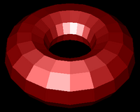
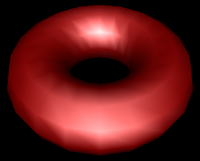
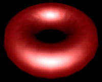
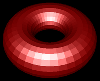
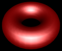
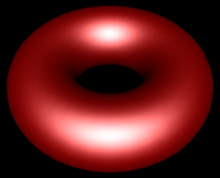
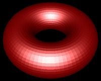
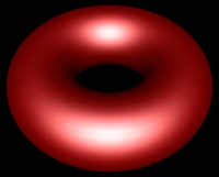
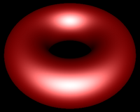
In last week's lab you saw these pictures. They show a full implementation of the Blinn-Phong reflection equation being applied in three different ways. The first is flat shading - one color is used for one whole primitive (triangle). The second is Gouraud shading - reflection is only calculated at the vertices, and colors are interpolated. The last is Phong shading - the full lighting equation is performed per fragment in the fragment shader. This week you will see results that look like all three columns, but you will always be doing Gouraud shading. You will add the Blinn-Phong specular component to a vertex shader, which produces the whitish highlight you see. The smoothness or flatness you will observe will be created entirely in the model - either by using the same normal for all vertices of a primitive (flat-like results) or high resolution meshes (Phong-like results).
| Flat Shading | Gouraud Shading | Phong Shading |
|---|---|---|
|
|
|
|
|
|
|
|
|
| Figure 3:Torus at different resolutions lit with Blinn-Phong reflection and shaded with different shading models. | ||
When you start to work with lighting, you move beyond color to normals, material properties and light properties. Normals describe what direction a surface is facing at a particular point. Material properties describe of what things are made of — or at least what they appear to be made of — by describing how they reflect light. Light properties describe the type and colour of the light interacting with the materials in the scene. Lights and materials can interact in many different ways. Describing these many different ways is one reason shaders are so important to modern 3D graphics APIs.
One common lighting model that relates geometry, materials and lights is the Blinn-Phong reflection model. It breaks lighting up into three simplified reflection components: diffuse, specular and ambient reflection. In this week's lab we will focus on specular reflection. The other two are left here for your reference.
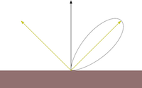
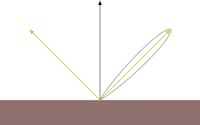
Specular reflection represents the shine that you see on very smooth or polished surfaces. Phong specular reflection takes into account both the angle between your eye and the direction the light would be reflected. As your eye approaches the direction of reflection, the apparent brightness increases. It assumes that light will be scattered toward the mirror reflection direction. A special shininess parameter (labelled α in the textbook, but s, here) is used to control how tight this scattering is. The Blinn-Phong specular reflection is very similar to Phong, but it fixes some technical shortcomings having to do with backscatter (compare the curves you see if figure 5). Instead of using the reflection vector it uses a vector that is halfway between the light and the eye. This vector is then compared to the normal.
The Blinn-Phong specular component is calculated by these equations:
h = (e+l)/|(e+l)|
Is = ms Ls (h · n)s
Where:
| Specular exponent | |||
|---|---|---|---|
| 1 | 10 | 100 | |
| Phong | 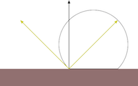 |
 |
 |
| Blinn-Phong | 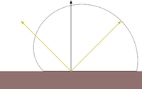 |
 |
 |
|
Figure 5: Phong vs Blinn-Phong With Varying Shininess Values. Both the Phong and Blinn-Phong reflectance functions cause a highlight to appear around the direction of reflection. Blinn-Phong has a fix that allows a near-diffuse disctribution at low shininess. Notice that at shininess 1 the Phong highlight would be invisible past 90° from the reflection direction, but Blinn-Phong is visible well past that point. Blinn-Phong also appears slightly more diffuse at all shininess values than Phong. |
|||

|
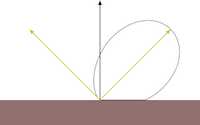
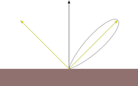
| Figure 6: Blinn-Phong at Varying Angles. |
Diffuse reflection is the more or less uniform scattering of light that you see in matte or non-shiny materials, like paper. The intensity that you see depends solely on the position of the light and the direction the surface is facing. The Blinn-Phong model calculates it using the Lambertian reflectance equation:
Id = md Ld (l · n)
Where:
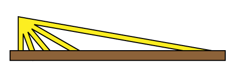
The dot product between l and n corresponds to the cosine of the angle between the two vectors. If they are the same, then the dot product is 1 and the diffuse reflection is brightest. As the angle increases toward 90° the dot product approaches 0, and the diffuse reflection gets dimmer. This change resembles the how a fixed width of light spreads out over a greater area when it hits a surface at different angles, as illustrated in Figure 4.
 |
|---|
| Figure 4: The same width of light covers a larger area as its angle to the surface normal increases. |
Even if the light does not reach a point on the surface directly, it may reach it by reflecting off of other surfaces in the scene. Rather than compute all the complex interreflections, we approximate this with ambient reflection. The ambient reflection is a simple product of the ambient colors of both the light and material. Direction does not factor in. The ambient reflectance equation is then:
Ia = ma La
Where:
A vertex shader that implements all of this is included in Demo 1 (see L5-1.html). Its code is shown below. The new specular lighting code is highlighted for your convenience:I = Is + Id + Ia
//diffuse and ambient multi-light shader

//inputs
attribute vec4 vPosition;
attribute vec3 vNormal;

//outputs
varying vec4 color;

//structs
struct _light
{
    vec4 diffuse;
    vec4 ambient;
    vec4 specular;
    vec4 position;
};

struct _material
{
    vec4 diffuse;
    vec4 ambient;
    vec4 specular;
    float shininess;
};

//constants
const int n = 1; // number of lights

//uniforms
uniform mat4 p;     // perspective matrix
uniform mat4 mv;    // modelview matrix
uniform bool lighting;  // to enable and disable lighting
uniform vec4 uColor;    // colour to use when lighting is disabled
uniform _light light[n]; // properties for the n lights
uniform _material material; // material properties

//globals
vec4 mvPosition; // unprojected vertex position
vec3 N; // fixed surface normal

//prototypes
vec4 lightCalc(in _light light);

void main()
{
  //Transform the point
  mvPosition = mv*vPosition;  //mvPosition is used often
  gl_Position = p*mvPosition;

  if (lighting == false)
  {
	color = uColor;
  }
  else
  {
    //Make sure the normal is actually unit length,
    //and isolate the important coordinates
    N = normalize((mv*vec4(vNormal,0.0)).xyz);

    //Combine colors from all lights
    color.rgb = vec3(0,0,0);
    for (int i = 0; i < n; i++)
    {
        color += lightCalc(light[i]);
    }
    color.a = 1.0; //Override alpha from light calculations
  }
}

vec4 lightCalc(in _light light)
{
  //Set up light direction for positional lights
  vec3 L;

  //If the light position is a vector, use that as the direction
  if (light.position.w == 0.0)
    L = normalize(light.position.xyz);
  //Otherwise, the direction is a vector from the current vertex to the light
  else
    L = normalize(light.position.xyz - mvPosition.xyz);

  //Set up eye vector
  vec3 E = -normalize(mvPosition.xyz);

  //Set up Blinn half vector
  vec3 H = normalize(L+E);

  //Calculate specular coefficient
  float Ks = pow(max(dot(N, H),0.0), material.shininess);

  //Calculate diffuse coefficient
  float Kd = max(dot(L,N), 0.0);

  //Calculate colour for this light
  vec4 color =  Ks * material.specular * light.specular
  			   + Kd * material.diffuse * light.diffuse
               + material.ambient * light.ambient;

  return color;
}
Appropriate changes should be made to get and set the specular color and shininess uniforms. The process is similar to what you observed with diffuse and ambient lighting.
Classic OpenGL has five material properties affect a material's illumination. They are introduced in the Blinn-Phong model section and implemented in the shaders in lab demo 2. They are explained below.
The steps are as follows:
Seeing the effects of varying material properties may help you select the ones you want.
In this week's first demo, L5-1, specular, diffuse and ambient material properties have been implemented. They have been declared for you globally, given default values and sent to the shader. The program provides convenient color pickers to allow you to select different specular and diffuse/ambient colors interactively. It also provides sliders to rotate the light about the Y-axis and change the shininess value. You should take some time to get familiar with the effects of the different properties.
Click here to view demo on its own.
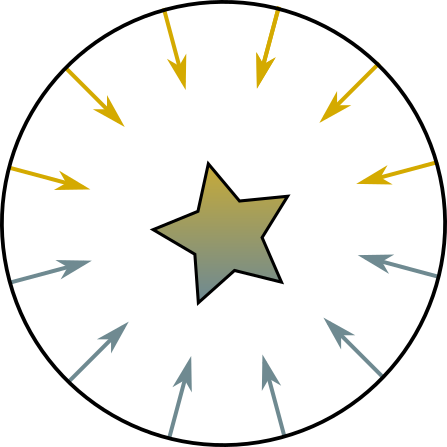
Specular lighting adds a lot to diffuse and ambient lighting as taught in the textbook. The ambient components are a hack to simulate global illumination, and they do a pretty poor job. Unless you use textures, there's no detail to be seen in ambient light - only a flat silhouette. Hemisphere lighting is a better looking hack that extends the light all around the object. It uses two colors of light, but each considered to be in opposite hemispheres shining toward the object. Toward the middle, the two colors blend smoothly. These colors are intended to represent the sky and the ground, but many implementations allow you to specify the direction of the north pole, or top hemisphere, so it becomes simple to specify directional, two color global illumination.
This picture illustrates the intent:
 |
|---|
| Figure 5: Hemisphere lighting's concept. Light falls on the object from two opposite hemispheres and blends across the object. |
Downward facing normals are lit entierly by the bottom hemisphere. Upward facing normals are lit entirely by the upper hemisphere. Angled normals are linearly blended (or "lerped") between the two, based on their angle to the "north pole" or top direction.
The proper equation for this is:
Color = a · TopColor + (1 - a) · BottomColor
Where:
a = 1.0 - (0.5 · sin(Θ)) for Θ ≤ 90°
a = (0.5 · sin(Θ)) for Θ > 90°
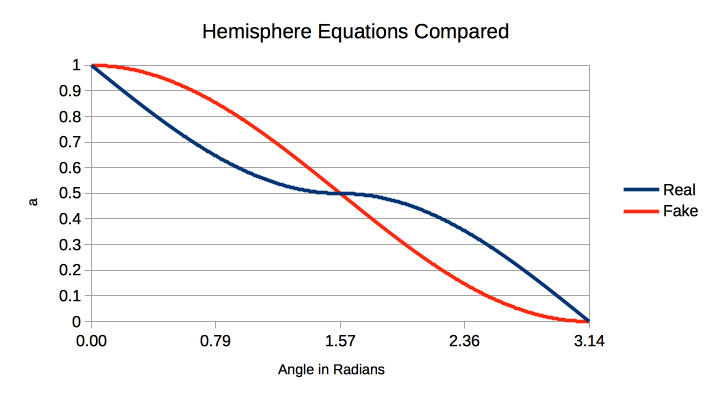
This can be simplified without too much error to:
a = 0.5 + (0.5 · cos(Θ))
Which replaces an expensive sin() with a cos() and saves a branch instruction. Remember that in WebGL shader programs both paths through a branch are always executed, so the elimination of the conditional can potential double the speed of this block of code. Since this method of global illumination is already approximate, the error is mostly harmless. Here are the two curves overlaid on each other:
 |
|---|
| Figure 6: Comparison of real vs. fake a calculation for hemisphere lighting. |
The following shader implements hemisphere lighting. You will find it in L5-2.html:
//hemisphere lighting shader with optional diffuse lighting path

//inputs
attribute vec4 vPosition;
attribute vec3 vNormal;

//outputs
varying vec4 color;

//structs
struct _light
{
    vec4 top;
    vec4 bottom;
    vec4 direction;
    bool hemisphere;  // to switch between hemisphere and directional lighting
};

struct _material
{
    vec4 diffuse;
};

//uniforms
uniform mat4 p;     // perspective matrix
uniform mat4 mv;    // modelview matrix


uniform _material material; // material properties
uniform _light light;		// light properties

//globals
vec4 mvPosition; // unprojected vertex position
vec3 N; // fixed surface normal

void main()
{
  //Transform the point
  mvPosition = mv*vPosition;  //mvPosition is used often
  gl_Position = p*mvPosition;

  //Make sure the normal is actually unit length,
  //and isolate the important coordinates
  N = normalize((mv*vec4(vNormal,0.0)).xyz);

  //Clean up light direction
  vec3 L;
  L = normalize(light.direction.xyz);

  //Calculate cosine of angle between light direction and normal
  float costheta = dot(L,N);

  //Calculate appropriate lighting colour
  if (light.hemisphere == true) //hemisphere technique
  {
  	float a = 0.5+(0.5*costheta);
  	color = a * light.top * material.diffuse
  	      + (1.0-a)* light.bottom * material.diffuse;
  }
  else	//lambertian technique with pseudo-ambient
  {
  	float Kd = max(costheta, 0.0);
  	color = Kd * material.diffuse * light.top
               + material.diffuse * light.bottom;
  }

  color.a = 1.0; //Override alpha from light calculations
}
And here is Lab 5 Demo 2, L5-2, for you to experiment with:
Observe how much detail you can make out in the shadows with Hemisphere Lighting as compared with Lambertian Directional Lighting. Notice, also, that the latter is brighter - this is because the ambient and diffuse colors are added rather than linearly blended.
In the real world a point light source, or positional light, will have less power to light an object the farther the two are apart. This is called attenuation. Because the light spreads out in an ever increasing sphere, the intensity of the light decreases in inverse proportion to the square of the distance. Classic OpenGL has three parameters to calculate the attenuation factor: constant, linear, and quadratic attenuation. These three factors are used as shown in this equation:
float attenuation = 1.0
if (/* light is positional */)
{
   float lightDistance = length(light.position.xyz - mvPosition.xyz);
   attenuation = 1.0/(constant + linear * lightDistance + quadratic * lightDistance^2);
}
In the above code, constant could be any positive float. Linear and quadratic are both factors in the range [0.0-1.0] indicating to what extent the attenuation involves linear and quadratic components. This calculation is applied separately to the entire color of each light - you multiply that light's color by the attenuation, something like this
// where color is the color result for one light
// and attenuation is 1 for directional lights
color = attenuation * color;
Attenuation is not implemented in the shaders in this week's lab. This is left for you to do as an exercise.
Before you begin, be sure you are using the Common folder from Lab5E.zip. This lab adds two important libraries - Apple's j3di.js, which provides an OBJ file loader, and East Desire's jscolor.js which provides the color picker you see in the demos. They are in this folder for your convenience.
Remember that for your program to be able to load OBJ files (such as the Batman model in this demo) from your file system you may have to start Chrome like this on a Mac:
open /Applications/Google\ Chrome.app --args --allow-file-access-from-files
Alternatively, you can run your program with Firefox.
Goals:
Instructions
/10