7. Markov Chains

In College Town, Pizza Company gets a lot of business. They get so many calls each night that they have to operate three kitchens to fill all the orders. They decided to spread the kitchens out so that each one is near one of the housing sections of the university. Since the same people own all three branches of Pizza Company, they only hired one set of delivery drivers to serve all three kitchens. After a driver makes a delivery, he or she goes to the nearest kitchen to pick up the next order. Therefore, the location of a delivery person's next order depends only on his or her present location. 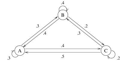The kitchens are logically named according to their area of campus. Of the calls to kitchen A, 30% are delivered in area A, 30% go to area B, and 40% go to area C. Of the orders placed at kitchen B, 40% go to area A, 40% go to area B, and 20% go to area C. Of the calls to kitchen C, 50% go to area A, 30% go to area B, and 20 go to area C. The picture below depicts the situation.

As you might guess, this information will be easier to read if we write it in matrix form. We will call this matrix S because it expresses the probability of movement (transition) from one state to the next. A state is the condition or location of an object in the system at a particular time. Therefore, our diagram is called a state diagram. Matrices of this type are called transition matrices. Our labeled transition matrix looks like this:

For each element, S_ij, i represents the starting location, and j represents the ending location for that move. This means that the row is the beginning location, and the column is the ending location after one move. We will want to learn things about what will happen in the future to Pizza Company, and this situation has the attributes necessary for what is called a Markov chain. Therefore, we will model the problem as a Markov chain in order to obtain information about the future.

A problem can be considered a (homogeneous) Markov chain if it has the following properties:

1. For each time period, every object (person) in the system is in exactly one of the defined states. At the end of each time period, each object either moves to a new state or stays in that same state for another period.

2. The objects move from one state to the next according to the transition probabilities which depend only on the current state (they do not take any previous history into account). The total probability of movement from a state (movement from a state to the same state does count as movement) must equal one.

3. The transition probabilities do not change over time (the probability of going from state A to state B today is the same as it will be at any time in the future).
   

Remark 19 Requirement (c) is not a requirement of Markov chains in general. It is a requirement for a special kind of Markov chain called a homogeneous Markov chain. We will be studying only homogeneous Markov chains in this book, so we will use the term Markov chain to refer to a homogeneous Markov chain.

The transition matrix used to model the Markov chain will have the following properties:

1. Each element of the transition matrix is a probability; therefore, each is a number between 0 and 1, inclusive.

2. The elements of each row of the transition matrix sum to 1. This is due to property (b) of a Markov chain.

3. The transition matrix must be square because it has a row and a column for each state.

Remark 20 Some assumptions are not completely accurate, but if we did not make assumptions to generalize the problem, we would not have the abitlity to approximate a solution to the problem. We just need to make sure that our assumptions are reasonable. The assumption that each delivery takes the same amount of time is reasonable if you consider that the average delivery times should be nearly equal.

Well, lets start with a simpler question. If you begin at kitchen C, what is the probability that you will be in area B after 2 deliveries? Think about how you can get to B. We can go from C to C, then from C to B. We can go from C to B, then from B to B. We can go from C to A, then from A to B. We will let P(CB) represent the probability of going from C to B in one delivery. Let's write this probability in our shorthand notation. Do you remember how probabilities work? If two (or more) independent events must both (all) happen, we multiply their probabilities together. If there are two (or more) distinct events that would both (all) work, we add the probabilities of those events together.

Remark 21 Notice that we said we can multiply probabilities together if the events are independent. We know that our events are independent of one another becasue someone in area A is equally likely to order a pizza whether or not someone in area B or C ordered pizza. If our events were not independent, we would not be able to simply multiply the probabilities.

You will notice that the elements on each row still add to 1 and each element is between 0 and 1, inclusive. Since we are modeling our problem with a Markov chain, this is essential. This matrix indicates the probabilities of going from kitchen i to kitchen j in exactly 2 deliveries.

Now that we have this matrix, it should be easier to find where we will be after 3 deliveries. We will let p(AB) represent the probability of going from A to B in 2 deliveries. Let's find the probability of going from C to B in 3 deliveries. The probability is p(CA)P(AB) + p(CB)P(BB) + p(CC)P(CB) = (.37)(.3) + (.33)(.4) + (.3)(.3) = .333. Where do these numbers come from? This probability is the inner product of row three of S² and column two of S. Therefore, if we multiply S² by S, we will get the probability matrix for 3 deliveries.

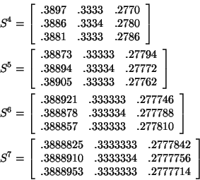
By now, you probably know how we find the matrix of probabilities for 4, 5 or more deliveries. Notice that the elements on each row still add to 1. Therefore, it is important that you do not round your answers. Keep as many decimal places as possible to retain accuracy.

What do you notice about these matrices as we take into account more and more deliveries? The numbers in each column seems to be converging to a particular number. Think about what this tells us about our long term probabilities. This tells us that after a large number of deliveries, it no longer matters which kitchen we were in when we started. At the end of the evening, we have a chance of being at kitchen A, chance of being at kitchen B, and Chance of being in kitchen C. This convergence will happen with most of the transition matrices that we consider.

Remark 22 If all the entries of the transition matrix are between 0 and 1 EXCLUSIVELY, then convergence is guaranteed to take place. Convergence may take place when 0 and 1 are in the transition matrix, but convergence is no longer guaranteed. For an example, look at the matrix Think about the situation that this marix represents in order to understand why A^k oscillates as k grows.

After the entire evening, we said that the fractions would converge to particular numbers so that the area from which we start doesn't matter. After many deliveries, we will obtain the same right-hand side no matter with which initial distribution we start. For example,

Notice that the right-hand side is the same as one of the rows of our transition matrix after many deliveries. This is exactly what we expected because we said that of the people will be in area A after many deliveries regardless of what percentage of the people were in area A in the initial distribution. Check this with several initial distributions to convince yourself of the truth of this statement.

If the initial distribution indicates the actual number of people in the system, our system can be represented by the following after one delivery:

Did you notice that we now have a fractional number of people in areas A and C after one delivery? We know that this cannot happen, but this gives us a good idea of approximately how many delivery people are in each area. After many deliveries, the right-hand side of this equality will also be very close to a particular vector. For example,

The particular vector that the product converges to is the total number of people in the system (54 in this case) times any row of the matrix that A^k converges to as k grows,

Try some examples to convince yourself that the vector indicating the number of people in each area after many deliveries will not change if people are moved from one state to another in the initial distribution. Also notice that the number of people in the entire system never changes. People move from place to place, but the system never loses or gains people.

Remark 23 It is usual to associate the word vector with a column vector, so a row vector is a transposed vector. Therfore, we will write

as x^TA = b^T and

as x^TA^k = b^T where k is a large whole number.

Remark 24 Some authors set up transition matrices so that j represents the starting location and i represents the ending location. In these cases the columns add to one. For this case, the entire equation is transposed, so instead of x^TA^k = b^T where x is the column vector of initial distribution and b is the column vector of distribution after k steps, the equation is (A^k)^Tx = b.